1.6 Harnack Curves

In 1876, Harnack [Har-76] not only proved the inequality 1.3.E in Section 1.3, but also completed the topological classification of nonsingular plane curves by proving the following theorem.

1.6.A Harnack Theorem.   For any natural number $m$ and any integer $c$ satisfying the inequalities

$$\frac {1-(-1)^m} 2 \le c\le\frac {m^2-3m+4}2,$$ (1)

there exists a nonsingular plane curve of degree $m$ consisting of $c$ components.

The inequality on the right in 1 is Harnack Inequality. The inequality on the left is part of Corollary 1 of Bézout's theorem (see Section 1.3.B). Thus, Harnack Theorem together with theorems 1.3.B and 1.3.E actually give a complete characterization of the set of topological types of nonsingular plane curves of degree $m$, i.e., they solve problem 1.1.A.

Curves with the maximum number of components (i.e., with $(m^2-3m+4)/2$ components, where $m$ is the degree) are called M-curves. Curves of degree $m$ which have $(m^2-3m+4)/2-a$ components are called $(M-a)$-curves. We begin the proof of Theorem 1.6.A by establishing that the Harnack Inequality 1.3.B is best possible.

1.6.B   For any natural number $m$ there exists an M-curve of degree $m$.

Proof. We shall actually construct a sequence of M-curves. At each step of the construction we add a line to the M-curve just constructed, and then give a slight perturbation to the union. We can begin the construction with a line or, as in Harnack's proof in [Har-76], with a circle. However, since we have already treated curves of degree $\le 5$ and constructed M-curves for those degrees (see Section 1.4), we shall begin by taking the M-curve of degree 5 that was constructed in Section 1.4, so that we can immediately proceed to curves that we have not encountered before.

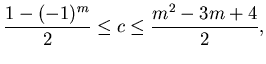
Recall that we obtained a degree 5 M-curve by perturbing the union of two conics and a line $L$. This perturbation can be done using various curves. For what follows it is essential that the auxiliary curve intersect $L$ in five points which are outside the two conics. For example, let the auxiliary curve be a union of five lines which satisfies this condition (Figure 6). We let $B_5$ denote this union, and we let $A_5$ denote the M-curve of degree 5 that is obtained using $B_5$.

Figure 6:

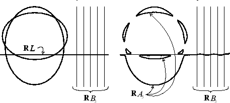
We now construct a sequence of auxiliary curves $B_m$ for $m>5$. We take $B_m$ to be a union of $m$ lines which intersect $L$ in $m$ distinct points lying, for even $m$, in an arbitrary component of the set $\mathbb{R}L\smallsetminus \mathbb{R}B_{m-1}$ and for odd $m$ in the component of $\mathbb{R}L\smallsetminus \mathbb{R}B_{m-1}$ containing $\mathbb{R}L\cap \mathbb{R}B_{m-2}$.

Figure 7:

We construct the M-curve $A_m$ of degree $m$ using small perturbation of the union $A_{m-1}\cup L$ directed to $B_m$. Suppose that the M-curve $A_{m-1}$ of degree $m-1$ has already been constructed, and suppose that $\mathbb{R}A_{m-1}$ intersects $\mathbb{R}L$ transversally in the $m-1$ points of the intersection $\mathbb{R}L\cap \mathbb{R}B_{m-1}$ which lie in the same component of the curve $\mathbb{R}A_{m-1}$ and in the same order as on $\mathbb{R}L$. It is not hard to see that, for one of the two possible directions of a small perturbation of $A_{m-1}\cup L$ directed to $B_m$, the line $\mathbb{R}L$ and the component of $\mathbb{R}A_{m-1}$ that it intersects give $m-1$ components, while the other components of $\mathbb{R}A_{m-1}$, of which, by assumption, there are

$$((m-1)^2-3(m-1)+4)/2-1=(m^2-5m+6)/2,$$

are only slightly deformed--so that the number of components of $\mathbb{R}A_m$ remains equal to $(m^2-5m+6)/2+m-1= (m^2-3m+4)/2$. We have thus obtained an M-curve of degree $m$. This curve is transversal to $\mathbb{R}L$, it intersects $\mathbb{R}L$ in $\mathbb{R}L\cap \mathbb{R}B_m$ (see 1.5.A), and, since $\mathbb{R}L\cap \mathbb{R}B_m$ is contained in one of the components of the set $\mathbb{R}L\smallsetminus \mathbb{R}B_{m-1}$, it follows that the intersection points of our curve with $\mathbb{R}L$ are all in the same component of the curve and are in the same order as on $\mathbb{R}L$ (Figure 7). $\qedsymbol$

The proof that the left inequality in 1 is best possible, i.e., that there is a curve with the minimum number of components, is much simpler. For example, we can take the curve given by the equation $x^m_0+x^m_1+x^m_2=0$. Its set of real points is obviously empty when $m$ is even, and when $m$ is odd the set of real points is homeomorphic to $\mathbb{R}P^1$ (we can get such a homeomorphism onto $\mathbb{R}P^1$, for example, by projection from the point $(0:0:1))$.

By choosing the auxiliary curves $B_m$ in different ways in the construction of M-curves in the proof of Theorem 1.6.B, we can obtain curves with any intermediate number of components. However, to complete the proof of Theorem 1.6.A in this way would be rather tedious, even though it would not require any new ideas. We shall instead turn to a less explicit, but simpler and more conceptual method of proof, which is based on objects and phenomena not encountered above.