1 Graphs of polynomials on logarithmic paper

1.1 How to visualize a real polynomial?

If you ever tried to draw the graph for a polynomial of degree greater than, say, 4 and consisting of at least 4 monomials, you are aware of the natural difficulties:
$\bullet$ The graph is too steep.
$\bullet$ Whatever scale you choose, either some important details do not fit into the picture or are too small.

The usual recipes from Calculus do not address the problem, but suggest, instead, to find roots of the first two derivatives, which does not seem to be much easier than the original problem.

1.2 Logarithmic paper

A physicist or engineer can give a more practical advice: use (double) logarithmic paper.

This is a graph paper, called also log paper, with a non-uniform net of coordinate lines and logarithmic scales on both axes. On a log paper a point with coordinates $x$, $y$ is shown at the position with the usual, Cartesian coordinates equal to $\ln x$, $\ln y$. In other words, the transition to the log paper corresponds to the change of coordinates:

$$\begin{cases}u=\ln x v=\ln y. \end{cases}$$

On a log paper the first quadrant is expanded homeomorphically to the whole plane, the line $x=1$ occupies the position of the axis of ordinates, the line $y=1$ occupies the position of the axis of abscissas, the unit square bounded by these lines and the coordinate axes occupies the whole third quadrant.

1.3 A monomial on logarithmic paper

Let us try to follow the advice.     The simplest special case to consider:    $y=ax^k$     (i.e., the graph of monomial $ax^k$). We are forced to consider only positive $x,y$ and hence assume $a$ to be positive as well.      Then

$$v=\ln y=\ln(ax^k)=k\ln x+\ln a=ku+\ln a=ku+b,$$

where we denote $\ln a$ by $b$. Now the curve which we want to draw is defined in the coordinates $u$ and $v$ by the equation $v=ku+b$. Everybody knows that this is the straight line with slope $k$ meeting the axis of ordinates (i.e., $v$-axis) at $(0,b)$.

1.4 Few slightly more complicated polynomials

First, consider a line $y=1+x$. Then

$$v=\ln y=\ln(1+x)=\ln(1+e^u).$$

See Figure 1, where the graph of $v=\ln(1+e^u)$ is shown together with lines $v=0$ and $v=u$, which represent on the log paper the monomials $1$ and $x$ involved in our polynomial $1+x$. The graph of $v=\ln(1+e^u)$ looks like the broken line $v=\max\{0,u\}$ with a smoothed corner: it goes along and above of this broken line getting very close to it as $\vert u\vert$ grows. For $\vert u\vert>4$ the difference becomes beyond the resolution.

Figure 1: Log paper graph of $1+x$

Here are two further examples: the quadratic polynomials $1+e^{\pm5}x+x^2$. Then

$$v=\ln(1+e^{\pm5}x+x^2)=\ln(1+e^{u\pm5}+e^{2u}).$$

See Figure 2.

Figure 2: Log paper graphs of $1+e^{5}x+x^2$ and $1+e^{-5}x+x^2$.

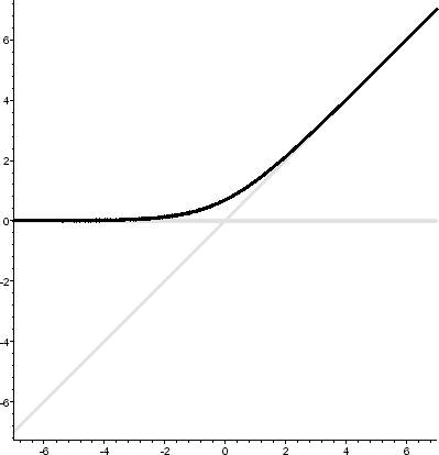
The graph of $v=\ln(1+e^{u\pm5}+e^{2u})$ looks like the broken line $v=\max\{0,u\pm5,2u\}$ with smoothed corners. It goes along and above of this broken line getting very close to it far from its corners. Notice that the lines $v=0$, $v=u\pm5$ and $v=2u$ represent on the logarithmic paper the monomials $1$, $e^{\pm5}x$ and $x^2$, respectively.

1.5 A polynomial versus the maximum of its monomials

This suggests, for a polynomial $p(x)=a_nx^{n}+a_{n-1}x^{n-1}+\dots+a_0$ with positive real coefficients $a_i=e^{b_i}$, to compare the graphs on log paper for $p$ and the maximum $M(p)(x)=\max\{a_nx^n,a_{n-1}x^{n-1},\dots,a_0\}$ of its monomials. Denote the graph on log paper of a function $f$ by $\Gamma _f$. With respect to the usual Cartesian coordinates, $\Gamma _p$ is the graph of

$$L_p(u)=\ln\left(e^{nu+b_n}+e^{(n-1)u+b_{n-1}}+\dots+e^{b_0}\right)$$

and $\Gamma _{M(p)}$ is the graph of a piecewise linear convex function

$$M_p(u)=\max\left\{nu+b_n, (n-1)u+b_{n-1}, \dots , b_0 \right\}.$$

Obviously, $M_p(u)\le L_p(u)\le M_p(u)+\ln(n+1)$. Hence $\Gamma _{p}$ is above $\Gamma _{M(p)}$, but below a copy of $\Gamma _{M(p)}$ shifted upwards by $\ln(n+1)$. The latter is in fact a rough estimate. It turns to equality only at $u$, where all linear functions, whose maximum is $M_p(u)$, are equal: $nu+b_n= (n-1)u+b_{n-1}=\dots=b_0$.

For a generic value of $u$, only one of these functions is equal to $M_p(u)$. Say $M_p(u)=ku+b_k$, while $M_p(u)>d+lu+b_l$ for some positive $d$ and each $l\ne k$. Then

$$L_p(u)<M_p(u)+\ln(1+ne^{-d})<M_p(u)+e^{-d}n.$$

If for some value of $u$ the values of all of the functions $ku+b_k$ except two are smaller than $M_p(u)-d$, then

$$L_p(u)<M_p(u)+\ln(2+(n-1)e^{-d})<M_p(u)+\ln2 +e^{-d}(n-1)/2.$$

Thus,    on a logarithmic paper the graph of a generic polynomial with positive coefficients lies in a narrow strip along the brocken line which is the graph of the maximum of its monomials. The width of the strip is estimated by characteristics of the mutual position of the lines which are the graphs of the monomials. The less congested the configuration of these lines, the norrower this strip.

1.6 Rescalings pushing the graph of a polynomial to a PL-graph

A natural way to make a configuration of lines less congested without changing its topology is to apply a dilation $(u,v)\mapsto(Cu,Cv)$ with a large $C>0$. In what follows it is more convenient to use instead of $C$ a parameter $h$ related to $C$ by $h=1/C$. (Surely, it is denoted by $h$ to hint to the Planck constant.) In terms of $h$ the dilation acts by $(u,v)\mapsto (u/h,v/h)$. It maps the graph of $v=ku+b$ to the graph of $v=ku+b/h$.

Notice, that the corresponding operation on monomials replaces $ax^{k}$ by $a^{1/h}x^{k}$.

Consider the corresponding family of polynomials: $p_{h}(x)=\sum_{k}a_k^{1/h}x^k$.    On log paper, the graphs of its monomials are obtained by dilation with ratio $1/h$ from the graphs of the corresponding monomials of $p$. Hence $\Gamma _{M(p_{h})}$ is the image of $\Gamma _{M(p)}$ under the same dilation. However, $\Gamma _{p_{h}}$ is not the image of $\Gamma _p$. It still lies in a strip along $\Gamma _{M(p_{h})}$ and the strip is getting narrower as $h$ decreases, but at the corners of $\Gamma _{M(p_{h})}$ the width of the strip cannot become smaller than $\ln2$.

To keep the picture of our expanding configuration of lines (the graphs of monomials) independent on $h$, let us make an additional calibration of coordinates: set $u_h=hu=h\ln x$,     $v_h=hv=h\ln y$. Denote by $\Gamma ^h_f$ the graph of a function $y=f(x)$ in the plane with coordinates $u_h, v_h$.

Then $\Gamma ^h_{M(p_{h})}$ does not depend on $h$. The additional scaling reduces the width of the strip along $\Gamma ^h_{M(p_h)}$, where $\Gamma ^h_{p_h}$ lies, forcing the width to tend to 0 as $h\to0$. Thus $\Gamma ^h_{p_{h}}$ tends to $\Gamma ^h_{M(p_h)}$ (in the $C^0$ sense) as $h\to0$.

The following graphs show how this happens if $p(x)=x^2+ex+1$.

The red curves are the graphs $\Gamma ^h_{p_h}$. They lie in the green strips along the convex PL-curve $\Gamma ^h_{M(p_{h})}$.