Initial data.
Let ![]() be a positive integer (it will be the degree of the curve
under construction) and
be a positive integer (it will be the degree of the curve
under construction) and ![]() be the triangle in
be the triangle in
![]() with vertices
with vertices
![]() ,
, ![]() ,
, ![]() . Let
. Let ![]() be a convex triangulation
of
be a convex triangulation
of ![]() with vertices having integer coordinates. The convexity of
with vertices having integer coordinates. The convexity of ![]() means that there exists a convex piecewise linear function
means that there exists a convex piecewise linear function
![]() which is linear on each triangle of
which is linear on each triangle of ![]() and
is not linear on the union of any two triangles of
and
is not linear on the union of any two triangles of ![]() . Let the
vertices of
. Let the
vertices of ![]() be equipped with signs. The sign (plus or minus) at
the vertex with coordinates
be equipped with signs. The sign (plus or minus) at
the vertex with coordinates ![]() is denoted by
is denoted by
![]() .
.
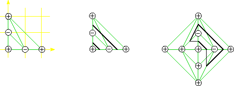
Construction of the piecewise linear curve.
If a triangle of the triangulation ![]() has vertices of different
signs, draw a midline separating pluses from minuses. Denote by
has vertices of different
signs, draw a midline separating pluses from minuses. Denote by ![]() the
union of these midlines. It is a collection of polygonal lines
contained in
the
union of these midlines. It is a collection of polygonal lines
contained in ![]() . The pair
. The pair
![]() is called the result of
combinatorial patchworking.
is called the result of
combinatorial patchworking.
Construction of polynomials.
Given initial data ![]() ,
, ![]() ,
, ![]() and
and
![]() as above and a positive
convex function
as above and a positive
convex function ![]() certifying, as above, that the triangulation
certifying, as above, that the triangulation
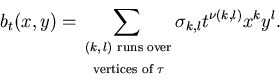
![]() is convex. Consider a one-parameter family of polynomials
is convex. Consider a one-parameter family of polynomials
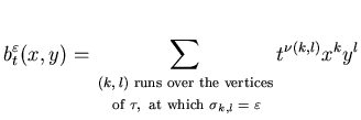
Patchwork Theorem. Let
![]() ,
, ![]() ,
, ![]() ,
,
![]() and
and ![]() be initial data as above.
Denote by
be initial data as above.
Denote by ![]() the polynomials obtained by the polynomial
patchworking of these initial data, and by
the polynomials obtained by the polynomial
patchworking of these initial data, and by ![]() the
PL-curve in
the
PL-curve in ![]() obtained from the same
initial data by combinatorial patchworking.
obtained from the same
initial data by combinatorial patchworking.
Then for all sufficiently small ![]() the polynomial
the polynomial
![]() defines in the first quadrant
defines in the first quadrant
![]() a curve
a curve ![]() such that the pair
such that the pair
![]() is homeomorphic to the pair
is homeomorphic to the pair
![]() .
.
 |
The Patchwork Theorem applied to ![]() ,
, ![]() and
and
![]() gives a similar topological description of the curve defined in the
other quadrants by
gives a similar topological description of the curve defined in the
other quadrants by ![]() with sufficiently small
with sufficiently small ![]() . The results can
be collected in the following natural combinatorial construction.
. The results can
be collected in the following natural combinatorial construction.
Construction of the PL-curve. Take copies
![]() ,
,
![]() ,
,
![]() of
of ![]() , where
, where
![]() are reflections with respect to the coordinate axes and
are reflections with respect to the coordinate axes and
![]() .
Denote by
.
Denote by ![]() the square
the square
![]() .
Extend the triangulation
.
Extend the triangulation ![]() to a symmetric triangulation of
to a symmetric triangulation of ![]() ,
and the distribution of signs
,
and the distribution of signs
![]() to a distribution at the vertices of the extended triangulation by
the following rule:
to a distribution at the vertices of the extended triangulation by
the following rule:
![]() , where
, where
![]() . In other words, passing from a vertex to its
mirror image with respect to an axis we preserve its sign if the
distance from the vertex to the axis is even, and change the sign if
the distance is odd.
. In other words, passing from a vertex to its
mirror image with respect to an axis we preserve its sign if the
distance from the vertex to the axis is even, and change the sign if
the distance is odd.
If a triangle of the triangulation of ![]() has vertices
of different signs, select (as above) a midline separating pluses from minuses.
Denote by
has vertices
of different signs, select (as above) a midline separating pluses from minuses.
Denote by ![]() the union of the selected
midlines. It is a collection of polygonal lines contained in
the union of the selected
midlines. It is a collection of polygonal lines contained in ![]() .
The pair
.
The pair
![]() is called the result of affine combinatorial
patchworking. Glue by
is called the result of affine combinatorial
patchworking. Glue by ![]() the sides of
the sides of ![]() . The resulting space
. The resulting space
![]() is homeomorphic to the real projective plane
is homeomorphic to the real projective plane
![]() . Denote
by
. Denote
by ![]() the image of
the image of ![]() in
in ![]() and call the pair
and call the pair
![]() the
result of projective combinatorial patchworking.
the
result of projective combinatorial patchworking.
Addendum to the Patchwork Theorem. Under the assumptions of Patchwork
Theorem above, for all sufficiently small ![]() there exist a
homeomorphism
there exist a
homeomorphism
![]() mapping
mapping ![]() onto the the affine
curve defined by
onto the the affine
curve defined by ![]() and a homeomorphism
and a homeomorphism
![]() mapping
mapping ![]() onto the projective closure of this affine curve.
onto the projective closure of this affine curve.
![\includegraphics[width=4in,clip]{harnack.eps}](img232.png)
![\includegraphics[width=4in,clip]{gudkov.eps}](img233.png)
![\includegraphics[clip]{f3.eps}](img234.png)
The polynomial ![]() defined by (5) is presented as
defined by (5) is presented as
![]() , where
, where
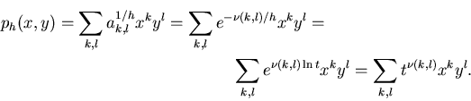
A monomial
![]() is presented in the
logarithmic space by the graph of
is presented in the
logarithmic space by the graph of
![]() . Hence the graph
of the maximum of linear forms corresponding to all monomials of
. Hence the graph
of the maximum of linear forms corresponding to all monomials of ![]() and
and ![]() is defined by
is defined by
Some of these faces correspond to monomials of ![]() , the others to
monomials of
, the others to
monomials of ![]() . The edges which separate the faces of these two
kinds constitute a broken line as in Section 3.4.
These edges are dual to the edges of
. The edges which separate the faces of these two
kinds constitute a broken line as in Section 3.4.
These edges are dual to the edges of ![]() which
intersect the result
which
intersect the result ![]() of the combinatorial patchworking.
of the combinatorial patchworking.
Therefore the topology of the projection to the ![]() -plane of
the broken line coincides with the topology of
-plane of
the broken line coincides with the topology of ![]() in
in ![]() .
.
We see that the quantum point of view (or its graphical log paper equivalent) gives a natural explanation to the simplest patchwork construction. The proofs become more conceptual and straight-forward. Of course, similar but slightly more involved quantum explanations can be given to all versions of patchwork.
Let me shortly mention other problems which can be attacked using similar arguments.
First of all, this is the Fewnomial Problem. Although A. G. Khovansky [3] proved that basically all topological characteristics of a real algebraic variety can be estimated in terms of the number of monomials in the equations, the known estimates seem to be far weaker than conjectures. For varieties classical from the quantum point of view a strong estimates are obvious. It is very compelling to estimate how much the topology can be complicated by the quantizing deformations.
There seem to be deep relations between the dequantization of algebraic geometry considered above and the results of I. M. Gelfand, M. M. Kapranov and A. V. Zelevinsky on discriminants [1]. In particular, some monomials in a discriminant are related to intersections of hyperplanes in the dequantized polynomial.
Complex algebraic geometry also deserves a dequantization. Especially relevant may be amoebas introduced in [1].