A connected curve can be situated in
![]() in two topologically distinct
ways: two-sidedly, i.e., as the boundary of a disc in
in two topologically distinct
ways: two-sidedly, i.e., as the boundary of a disc in
![]() ,
and one-sidedly, i.e., as a projective line. A two-sided
connected curve is called an oval. The complement of an oval in
,
and one-sidedly, i.e., as a projective line. A two-sided
connected curve is called an oval. The complement of an oval in
![]() has two components, one of which is homeomorphic to a disc and
the other homeomorphic to a Möbius strip. The first is called the
inside and the second is called the outside. The
complement of a connected one-sided curve is homeomorphic to a disc.
has two components, one of which is homeomorphic to a disc and
the other homeomorphic to a Möbius strip. The first is called the
inside and the second is called the outside. The
complement of a connected one-sided curve is homeomorphic to a disc.
Any two one-sided connected curves intersect, since each of them
realizes the nonzero element of the group
![]() ,
which has
nonzero self-intersection. Hence, a topological plane curve has at most
one one-sided component. The existence of such a component can be expressed in
terms of homology: it exists if and only if the curve represents a
nonzero element of
,
which has
nonzero self-intersection. Hence, a topological plane curve has at most
one one-sided component. The existence of such a component can be expressed in
terms of homology: it exists if and only if the curve represents a
nonzero element of
![]() . If it exists, then we
say that the whole curve is one-sided; otherwise, we say that the curve
is two-sided.
. If it exists, then we
say that the whole curve is one-sided; otherwise, we say that the curve
is two-sided.
Two disjoint ovals can be situated in two topologically distinct ways: each may lie outside the other one--i.e., each is in the outside component of the complement of the other--or else they may form an injective pair, i.e., one of them is in the inside component of the complement of the other--in that case, we say that the first is the inner oval of the pair and the second is the outer oval. In the latter case we also say that the outer oval of the pair envelopes the inner oval.
A set of ![]() ovals of a curve any two of which form an injective pair is
called a nest of depth
ovals of a curve any two of which form an injective pair is
called a nest of depth ![]() .
.
The pair
![]() , where
, where ![]() is a topological plane curve, is
determined up to homeomorphism by whether or not
is a topological plane curve, is
determined up to homeomorphism by whether or not ![]() has a one-sided component
and by the relative location of each pair of ovals. We shall adopt the
following
notation to describe this. A curve consisting of a single oval will be denoted
by the symbol
has a one-sided component
and by the relative location of each pair of ovals. We shall adopt the
following
notation to describe this. A curve consisting of a single oval will be denoted
by the symbol
![]() . The empty curve will be denoted by
. The empty curve will be denoted by
![]() . A one-sided connected curve will be denoted by
. A one-sided connected curve will be denoted by
![]() . If
. If
![]() is the symbol for a certain two-sided curve,
then the curve obtained by adding a new oval which envelopes all
of the other
ovals will be denoted by
is the symbol for a certain two-sided curve,
then the curve obtained by adding a new oval which envelopes all
of the other
ovals will be denoted by
![]() . A curve which is a
union of two disjoint curves
. A curve which is a
union of two disjoint curves
![]() and
and
![]() having
the property that none of the ovals in one curve is contained in an oval of the
other is denoted by
having
the property that none of the ovals in one curve is contained in an oval of the
other is denoted by
![]() . In addition, we use the
following
abbreviations: if
. In addition, we use the
following
abbreviations: if
![]() denotes a certain curve, and if a part of
another curve has the form
denotes a certain curve, and if a part of
another curve has the form
![]() , where
, where ![]() occurs
occurs
![]() times, then we let
times, then we let ![]() denote
denote
![]() . We further
write
. We further
write ![]() simply as
simply as ![]() .
.
When depicting a topological plane curve one usually represents the projective
plane either as a disc with opposite points of the boundary identified, or else
as the compactification of
![]() , i.e., one visualizes the curve as its
preimage under either the projection
, i.e., one visualizes the curve as its
preimage under either the projection
![]() or the inclusion
or the inclusion
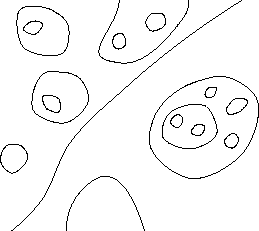
![]() . In this book we shall use the second method. For
example, 1.2 shows a curve corresponding to the symbol
. In this book we shall use the second method. For
example, 1.2 shows a curve corresponding to the symbol
![]() .
.