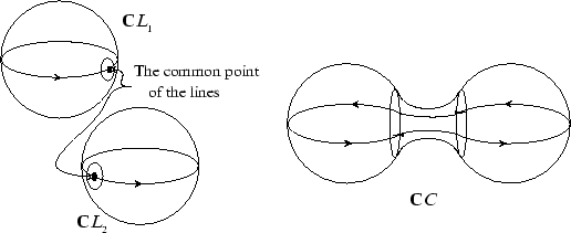
First, consider the simplest special case: a small perturbation
of the union of two real lines. Denote the lines by ![]() and
and ![]() and
the result by
and
the result by ![]() . As we saw above,
. As we saw above,
![]() and
and
![]() are
homeomorphic to
are
homeomorphic to ![]() . The spheres
. The spheres
![]() and
and
![]() intersect each
other at a single point. By the complex version of the implicit
function theorem,
intersect each
other at a single point. By the complex version of the implicit
function theorem,
![]() approximates
approximates
![]() outside a
neighborhood
outside a
neighborhood ![]() of this point in the sense that
of this point in the sense that
![]() is
a section of a tulubular neighborhood
is
a section of a tulubular neighborhood ![]() of
of
![]() , cf. 1.5.A. Thus
, cf. 1.5.A. Thus
![]() may be presented as
the union of two discs and a part contained in a small neighborhood of
may be presented as
the union of two discs and a part contained in a small neighborhood of
![]() . Since the whole
. Since the whole
![]() is homeomorphic to
is homeomorphic to ![]() and
the complement of two disjoint discs embedded into
and
the complement of two disjoint discs embedded into ![]() is
homeomorphic to the annulus, the third part of
is
homeomorphic to the annulus, the third part of
![]() is an annulus.
The discs are the complements
of a neighborhood of
is an annulus.
The discs are the complements
of a neighborhood of
![]() in
in
![]() and
and
![]() ,
respectively, slightly perturbed in
,
respectively, slightly perturbed in
![]() , and the annulus connects
the discs through the neighborhood
, and the annulus connects
the discs through the neighborhood ![]() of
of
![]() .
.
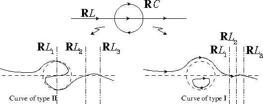
This is the complex view of the picture. Up to this point it does not matter whether the curves are defined by real equations or not.
To relate this to the real view presented in Section 1.5, one
needs to describe the position of the real parts of the curves in
their complexifications and the action of ![]() .
It can be recovered by rough topological
agruments. The whole complex picture above is invariant under
.
It can be recovered by rough topological
agruments. The whole complex picture above is invariant under
![]() . This means that the intersection point of
. This means that the intersection point of
![]() and
and
![]() is real, its neighborhood
is real, its neighborhood ![]() can be chosen to be
invariant under
can be chosen to be
invariant under ![]() . Thus each half of
. Thus each half of
![]() is presented as the
union of two half-discs and a half of the annulus: the half-discs
approximate the halves of
is presented as the
union of two half-discs and a half of the annulus: the half-discs
approximate the halves of
![]() and
and
![]() and a half of annulus is
contained in
and a half of annulus is
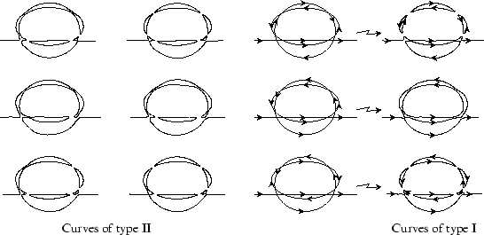
contained in ![]() . See Figure 15.
. See Figure 15.
This is almost complete description. It misses only one point: one has to specify which half-discs are connected with each other by a half-annulus.
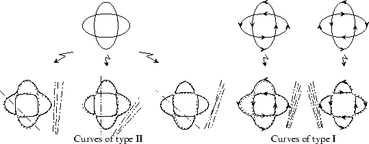
First, observe, that the halves of the complex point set of any curve of type I can be distinguished by the orientations of the real part. Each of the halves has the canonical orientation defined by the complex structure, and this orientation induces an orientation on the boundary of the half. This is one of the complex orientations. The other complex orientation comes from the other half. Hence the halves of the complexification are in one-to-one correspondence to the complex orientations.
Now we have an easy answer to the question above.
The halves of
![]() which are connected with each other after the
perturbation correspond to the complex orientations of
which are connected with each other after the
perturbation correspond to the complex orientations of
![]() which
agree with some orientation of
which
agree with some orientation of
![]() . Indeed, the perturbed union
. Indeed, the perturbed union
![]() of the lines
of the lines ![]() is a curve of type I (since this is a nonempty
conic, see Section 2.2). Each orientation of its real part
is a curve of type I (since this is a nonempty
conic, see Section 2.2). Each orientation of its real part
![]() is a complex orientation. Choose one of the orientations. It is
induced by the canonical orientation of a half of the complex point set
is a complex orientation. Choose one of the orientations. It is
induced by the canonical orientation of a half of the complex point set
![]() . Its restriction to the part of the
. Its restriction to the part of the
![]() obtained from
obtained from
![]() is induced by the orientation of the corresponding part of this
half.
is induced by the orientation of the corresponding part of this
half.
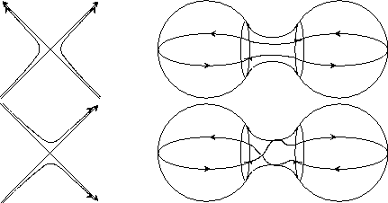
The union of two lines can be perturbed in two different ways. On the other hand, there are two ways to connect the halves of their complexifications. It is easy to see that different connections correspond to different perturbations. See Figure 16.
The special classical small perturbation considered above is a key for
understanding what happens in the complex domain at an arbitrary
classical small perturbation. First, look at the complex picture,
forgetting about the real part. Take a plane projective curve, which
has only nondegenerate double points. Near such a point it is organized
as a union of two lines intersecting at the point. This means that there
are a neighborhood ![]() of the point in
of the point in
![]() and a diffeomorphism of
and a diffeomorphism of
![]() onto
onto
![]() mapping the intersection of
mapping the intersection of ![]() and the curve onto a
union of two complex lines, which meet each other in 0. This follows
from the complex version of the Morse lemma. By the same Morse lemma,
near each double point the classical small perturbation is organized as
a small perturbation of the union of two lines: the union of two
transversal disks is replaced by an annulus.
and the curve onto a
union of two complex lines, which meet each other in 0. This follows
from the complex version of the Morse lemma. By the same Morse lemma,
near each double point the classical small perturbation is organized as
a small perturbation of the union of two lines: the union of two
transversal disks is replaced by an annulus.
For example, take the union of ![]() projective lines, no three of which
have a common point. Its complex point set is the union of
projective lines, no three of which
have a common point. Its complex point set is the union of ![]() copies of
copies of ![]() such that any two of them have exactly one common
point. A perturbation can be thought of as removal from each sphere
such that any two of them have exactly one common
point. A perturbation can be thought of as removal from each sphere
![]() disjoint discs and insertion
disjoint discs and insertion
![]() tubes connecting
the boundary circles of the disks removed. The result is orientable
(since it is a complex manifold). It is easy to realize that this is a
sphere with
tubes connecting
the boundary circles of the disks removed. The result is orientable
(since it is a complex manifold). It is easy to realize that this is a
sphere with
![]() handles. One may prove this counting
the Euler characteristic, but it may be seen directly: first, by inserting
the tubes which join one of the lines with all other lines we get a
sphere, then each additional tube gives rise to a handle. The
number of these handles is
handles. One may prove this counting
the Euler characteristic, but it may be seen directly: first, by inserting
the tubes which join one of the lines with all other lines we get a
sphere, then each additional tube gives rise to a handle. The
number of these handles is
By the way, this description shows that the complex point set of a
nonsingular plane projective curve of degree ![]() realizes the same
homology class as the union of
realizes the same
homology class as the union of ![]() complex projective lines: the
complex projective lines: the
![]() -fold generator of
-fold generator of
![]() .
.
Now let us try to figure out what happens with the complex schemes in an arbitrary classical small perturbation of real algebraic curves. The general case requirs some technique. Therefore we restrict ourselves to the following intermediate assertion.
If it takes place, then the orientation of
![]() is one
of the complex orientations of
is one
of the complex orientations of ![]() .
.
Assume now that all ![]() are of type I. If
are of type I. If ![]() is also of type I then
a half of
is also of type I then
a half of
![]() is obtained from halves of
is obtained from halves of
![]() as in the case
considered above. The orientation induced on
as in the case
considered above. The orientation induced on
![]() by the orientation
of the half agrees with orientations induced from the halves of the
corresponding pieces. Thus a complex orietation of
by the orientation
of the half agrees with orientations induced from the halves of the
corresponding pieces. Thus a complex orietation of ![]() agrees with
complex orientations of
agrees with
complex orientations of ![]() 's.
's.
Again assume that all ![]() are of type I. Let some complex
orientations of
are of type I. Let some complex
orientations of ![]() agree with a single orientation of
agree with a single orientation of
![]() . As it
follows from the Morse Lemma, at each intersection point the
perturbation is organized as the model perturbation considered above.
Thus the halves of
. As it
follows from the Morse Lemma, at each intersection point the
perturbation is organized as the model perturbation considered above.
Thus the halves of
![]() 's defining the complex orientations are
connected. It cannot happen that some of the halves will be connected
by a chain of halves to its image under
's defining the complex orientations are
connected. It cannot happen that some of the halves will be connected
by a chain of halves to its image under ![]() . But that would be the
only chance to get a curve of type II, since in a curve of type II each
imaginary point can be connected with its image under
. But that would be the
only chance to get a curve of type II, since in a curve of type II each
imaginary point can be connected with its image under ![]() by a path
disjoint from the real part.
by a path
disjoint from the real part. ![]()